Bernoulli mixture model

This example considers data generated from a Bernoulli mixture model. One simple example process could be a questionnaire for election candidates. We observe a set of binary vectors, where each vector represents a candidate in the election and each element in these vectors correspond to a candidate’s answer to a yes-or-no question. The goal is to find groups of similar candidates and analyze the answer patterns of these groups.

Data

First, we generate artificial data to analyze. Let us assume that the questionnaire contains ten yes-or-no questions. We assume that there are three groups with similar opinions. These groups could represent parties. These groups have the following answering patterns, which are represented by vectors with probabilities of a candidate answering yes to the questions:

>>> p0 = [0.1, 0.9, 0.1, 0.9, 0.1, 0.9, 0.1, 0.9, 0.1, 0.9]
>>> p1 = [0.1, 0.1, 0.1, 0.1, 0.1, 0.9, 0.9, 0.9, 0.9, 0.9]
>>> p2 = [0.9, 0.9, 0.9, 0.9, 0.9, 0.1, 0.1, 0.1, 0.1, 0.1]

Thus, the candidates in the first group are likely to answer no to questions 1, 3, 5, 7 and 9, and yes to questions 2, 4, 6, 8, 10. The candidates in the second group are likely to answer yes to the last five questions, whereas the candidates in the third group are likely to answer yes to the first five questions. For convenience, we form a NumPy array of these vectors:

>>> import numpy as np
>>> p = np.array([p0, p1, p2])

Next, we generate a hundred candidates. First, we randomly select the group for each candidate:

>>> from bayespy.utils import random
>>> z = random.categorical([1/3, 1/3, 1/3], size=100)

Using the group patterns, we generate yes-or-no answers for the candidates:

>>> x = random.bernoulli(p[z])

This is our simulated data to be analyzed.

Model

Now, we construct a model for learning the structure in the data. We have a dataset of hundred 10-dimensional binary vectors:

>>> N = 100
>>> D = 10

We will create a Bernoulli mixture model. We assume that the true number of groups is unknown to us, so we use a large enough number of clusters:

>>> K = 10

We use the categorical distribution for the group assignments and give the group assignment probabilities an uninformative Dirichlet prior:

>>> from bayespy.nodes import Categorical, Dirichlet
>>> R = Dirichlet(K*[1e-5],
...               name='R')
>>> Z = Categorical(R,
...                 plates=(N,1),
...                 name='Z')

Each group has a probability of a yes answer for each question. These probabilities are given beta priors:

>>> from bayespy.nodes import Beta
>>> P = Beta([0.5, 0.5],
...          plates=(D,K),
...          name='P')

The answers of the candidates are modelled with the Bernoulli distribution:

>>> from bayespy.nodes import Mixture, Bernoulli
>>> X = Mixture(Z, Bernoulli, P)

Here, Z defines the group assignments and P the answering probability patterns for each group. Note how the plates of the nodes are matched: Z has plates (N,1) and P has plates (D,K), but in the mixture node the last plate axis of P is discarded and thus the node broadcasts plates (N,1) and (D,) resulting in plates (N,D) for X.

Inference

In order to infer the variables in our model, we construct a variational Bayesian inference engine:

>>> from bayespy.inference import VB
>>> Q = VB(Z, R, X, P)

This also gives the default update order of the nodes. In order to find different groups, they must be initialized differently, thus we use random initialization for the group probability patterns:

>>> P.initialize_from_random()

We provide our simulated data:

>>> X.observe(x)

Now, we can run inference:

>>> Q.update(repeat=1000)
Iteration 1: loglike=-6.872145e+02 (... seconds)
...
Iteration 17: loglike=-5.236921e+02 (... seconds)
Converged at iteration 17.

The algorithm converges in 17 iterations.

Results

Now we can examine the approximate posterior distribution. First, let us plot the group assignment probabilities:

>>> import bayespy.plot as bpplt
>>> bpplt.hinton(R)

(Source code, png, hires.png, pdf)

This plot shows that there are three dominant groups, which is equal to the true number of groups used to generate the data. However, there are still two smaller groups as the data does not give enough evidence to prune them out. The yes-or-no answer probability patterns for the groups can be plotted as:

>>> bpplt.hinton(P)

(Source code, png, hires.png, pdf)

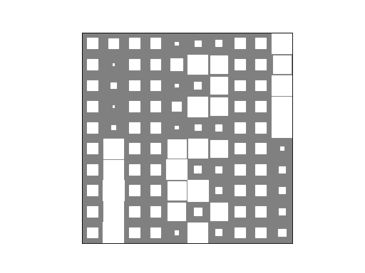
The three dominant groups have found the true patterns accurately. The patterns of the two minor groups some kind of mixtures of the three groups and they exist because the generated data happened to contain a few samples giving evidence for these groups. Finally, we can plot the group assignment probabilities for the candidates:

>>> bpplt.hinton(Z)

(Source code, png, hires.png, pdf)

This plot shows the clustering of the candidates. It is possible to use HintonPlotter to enable monitoring during the VB iteration by providing plotter=HintonPlotter() for Z, P and R when creating the nodes.