Gaussian mixture model
This example demonstrates the use of Gaussian mixture model for flexible density estimation, clustering or classification.
Data
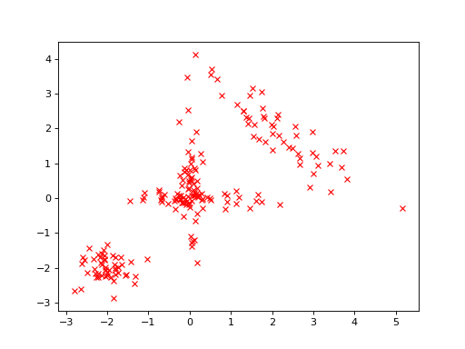
First, let us generate some artificial data for the analysis. The data are two-dimensional vectors from one of the four different Gaussian distributions:
>>> import numpy as np
>>> y0 = np.random.multivariate_normal([0, 0], [[2, 0], [0, 0.1]], size=50)
>>> y1 = np.random.multivariate_normal([0, 0], [[0.1, 0], [0, 2]], size=50)
>>> y2 = np.random.multivariate_normal([2, 2], [[2, -1.5], [-1.5, 2]], size=50)
>>> y3 = np.random.multivariate_normal([-2, -2], [[0.5, 0], [0, 0.5]], size=50)
>>> y = np.vstack([y0, y1, y2, y3])
Thus, there are 200 data vectors in total. The data looks as follows:
>>> import bayespy.plot as bpplt
>>> bpplt.pyplot.plot(y[:,0], y[:,1], 'rx')
[<matplotlib.lines.Line2D object at 0x...>]
(Source code, png, hires.png, pdf)

Model
For clarity, let us denote the number of the data vectors with N
>>> N = 200
and the dimensionality of the data vectors with D:
>>> D = 2
We will use a “large enough” number of Gaussian clusters in our model:
>>> K = 10
Cluster assignments Z and the prior for the cluster assignment probabilities
alpha:
>>> from bayespy.nodes import Dirichlet, Categorical
>>> alpha = Dirichlet(1e-5*np.ones(K),
...                   name='alpha')
>>> Z = Categorical(alpha,
...                 plates=(N,),
...                 name='z')
The mean vectors and the precision matrices of the clusters:
>>> from bayespy.nodes import Gaussian, Wishart
>>> mu = Gaussian(np.zeros(D), 1e-5*np.identity(D),
...               plates=(K,),
...               name='mu')
>>> Lambda = Wishart(D, 1e-5*np.identity(D),
...                  plates=(K,),
...                  name='Lambda')
If either the mean or precision should be shared between clusters, then that
node should not have plates, that is, plates=(). The data vectors are from
a Gaussian mixture with cluster assignments Z and Gaussian component
parameters mu and Lambda:
>>> from bayespy.nodes import Mixture
>>> Y = Mixture(Z, Gaussian, mu, Lambda,
...             name='Y')
>>> Z.initialize_from_random()
>>> from bayespy.inference import VB
>>> Q = VB(Y, mu, Lambda, Z, alpha)
Inference
Before running the inference algorithm, we provide the data:
>>> Y.observe(y)
Then, run VB iteration until convergence:
>>> Q.update(repeat=1000)
Iteration 1: loglike=-1.402345e+03 (... seconds)
...
Iteration 61: loglike=-8.888464e+02 (... seconds)
Converged at iteration 61.
The algorithm converges very quickly. Note that the default update order of the
nodes was such that mu and Lambda were updated before Z, which is
what we wanted because Z was initialized randomly.
Results
For two-dimensional Gaussian mixtures, the mixture components can be plotted
using gaussian_mixture_2d():
>>> bpplt.gaussian_mixture_2d(Y, alpha=alpha, scale=2)
The function is called with scale=2 which means that each ellipse shows two
standard deviations. From the ten cluster components, the model uses
effectively the correct number of clusters (4). These clusters capture the true
density accurately.
In addition to clustering and density estimation, this model could also be used for classification by setting the known class assignments as observed.
Advanced next steps
Joint node for mean and precision
The next step for improving the results could be to use GaussianWishart
node for modelling the mean vectors mu and precision matrices Lambda
jointly without factorization. This should improve the accuracy of the
posterior approximation and the speed of the VB estimation. However, the
implementation is a bit more complex.