Linear state-space model¶

Model¶

In linear state-space models a sequence of $M$ -dimensional observations $\mathbf{Y}=(\mathbf{y}_1,\ldots,\mathbf{y}_N)$ is assumed to be generated from latent $D$ -dimensional states $\mathbf{X}=(\mathbf{x}_1,\ldots,\mathbf{x}_N)$ which follow a first-order Markov process:

$\begin{aligned} \mathbf{x}_{n} &= \mathbf{A}\mathbf{x}_{n-1} + \text{noise} \,, \\ \mathbf{y}_{n} &= \mathbf{C}\mathbf{x}_{n} + \text{noise} \,, \end{aligned}$

where the noise is Gaussian, $\mathbf{A}$ is the $D\times D$ state dynamics matrix and $\mathbf{C}$ is the $M\times D$ loading matrix. Usually, the latent space dimensionality $D$ is assumed to be much smaller than the observation space dimensionality $M$ in order to model the dependencies of high-dimensional observations efficiently.

In order to construct the model in BayesPy, first import relevant nodes:

>>> from bayespy.nodes import GaussianARD, GaussianMarkovChain, Gamma, Dot

The data vectors will be 30-dimensional:

>>> M = 30

There will be 400 data vectors:

>>> N = 400

Let us use 10-dimensional latent space:

>>> D = 10

The state dynamics matrix $\mathbf{A}$ has ARD prior:

>>> alpha = Gamma(1e-5,
...               1e-5,
...               plates=(D,),
...               name='alpha')
>>> A = GaussianARD(0,
...                 alpha,
...                 shape=(D,),
...                 plates=(D,),
...                 name='A')

Note that $\mathbf{A}$ is a $D\times{}D$ -dimensional matrix. However, in BayesPy it is modelled as a collection (plates=(D,)) of $D$ -dimensional vectors (shape=(D,)) because this is how the variables factorize in the posterior approximation of the state dynamics matrix in GaussianMarkovChain. The latent states are constructed as

>>> X = GaussianMarkovChain(np.zeros(D),
...                         1e-3*np.identity(D),
...                         A,
...                         np.ones(D),
...                         n=N,
...                         name='X')

where the first two arguments are the mean and precision matrix of the initial state, the third argument is the state dynamics matrix and the fourth argument is the diagonal elements of the precision matrix of the innovation noise. The node also needs the length of the chain given as the keyword argument n=N. Thus, the shape of this node is (N,D).

The linear mapping from the latent space to the observation space is modelled with the loading matrix which has ARD prior:

>>> gamma = Gamma(1e-5,
...               1e-5,
...               plates=(D,),
...               name='gamma')
>>> C = GaussianARD(0,
...                 gamma,
...                 shape=(D,),
...                 plates=(M,1),
...                 name='C')

Note that the plates for C are (M,1), thus the full shape of the node is (M,1,D). The unit plate axis is added so that C broadcasts with X when computing the dot product:

>>> F = Dot(C,
...         X,
...         name='F')

This dot product is computed over the $D$ -dimensional latent space, thus the result is a $M\times{}N$ -dimensional matrix which is now represented with plates (M,N) in BayesPy:

>>> F.plates
(30, 400)

We also need to use random initialization either for C or X in order to find non-zero latent space because by default both C and X are initialized to zero because of their prior distributions. We use random initialization for C and then we must update X the first time before updating C:

>>> C.initialize_from_random()

The precision of the observation noise is given gamma prior:

>>> tau = Gamma(1e-5,
...             1e-5,
...             name='tau')

The observations are noisy versions of the dot products:

>>> Y = GaussianARD(F,
...                 tau,
...                 name='Y')

The variational Bayesian inference engine is then construced as:

>>> from bayespy.inference import VB
>>> Q = VB(X, C, gamma, A, alpha, tau, Y)

Note that X is given before C, thus X is updated before C by default.

Data¶

Now, let us generate some toy data for our model. Our true latent space is four dimensional with two noisy oscillator components, one random walk component and one white noise component.

>>> w = 0.3
>>> a = np.array([[np.cos(w), -np.sin(w), 0, 0],
...               [np.sin(w), np.cos(w),  0, 0],
...               [0,         0,          1, 0],
...               [0,         0,          0, 0]])

The true linear mapping is just random:

>>> c = np.random.randn(M,4)

Then, generate the latent states and the observations using the model equations:

>>> x = np.empty((N,4))
>>> f = np.empty((M,N))
>>> y = np.empty((M,N))
>>> x[0] = 10*np.random.randn(4)
>>> f[:,0] = np.dot(c,x[0])
>>> y[:,0] = f[:,0] + 3*np.random.randn(M)
>>> for n in range(N-1):
...     x[n+1] = np.dot(a,x[n]) + [1,1,10,10]*np.random.randn(4)
...     f[:,n+1] = np.dot(c,x[n+1])
...     y[:,n+1] = f[:,n+1] + 3*np.random.randn(M)

We want to simulate missing values, thus we create a mask which randomly removes 80% of the data:

>>> from bayespy.utils import random
>>> mask = random.mask(M, N, p=0.2)
>>> Y.observe(y, mask=mask)

Inference¶

As we did not define plotters for our nodes when creating the model, it is done now for some of the nodes:

>>> import bayespy.plot as bpplt
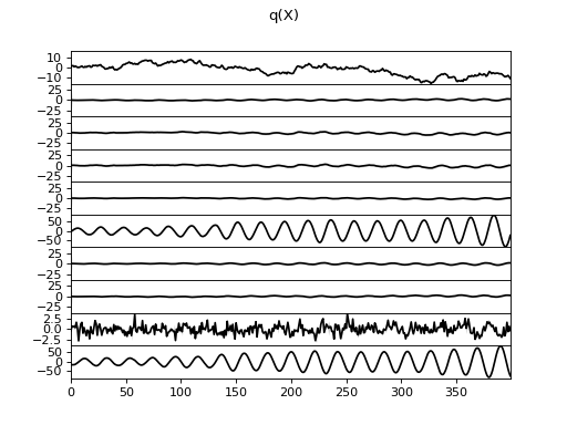
>>> X.set_plotter(bpplt.FunctionPlotter(center=True, axis=-2))
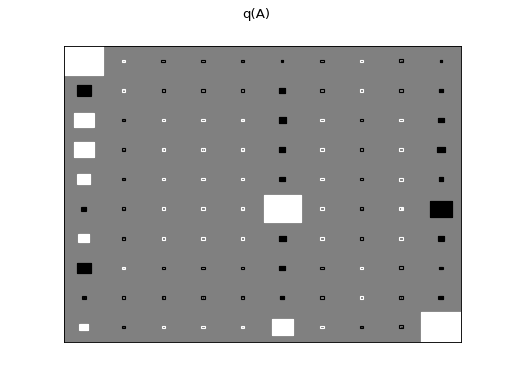
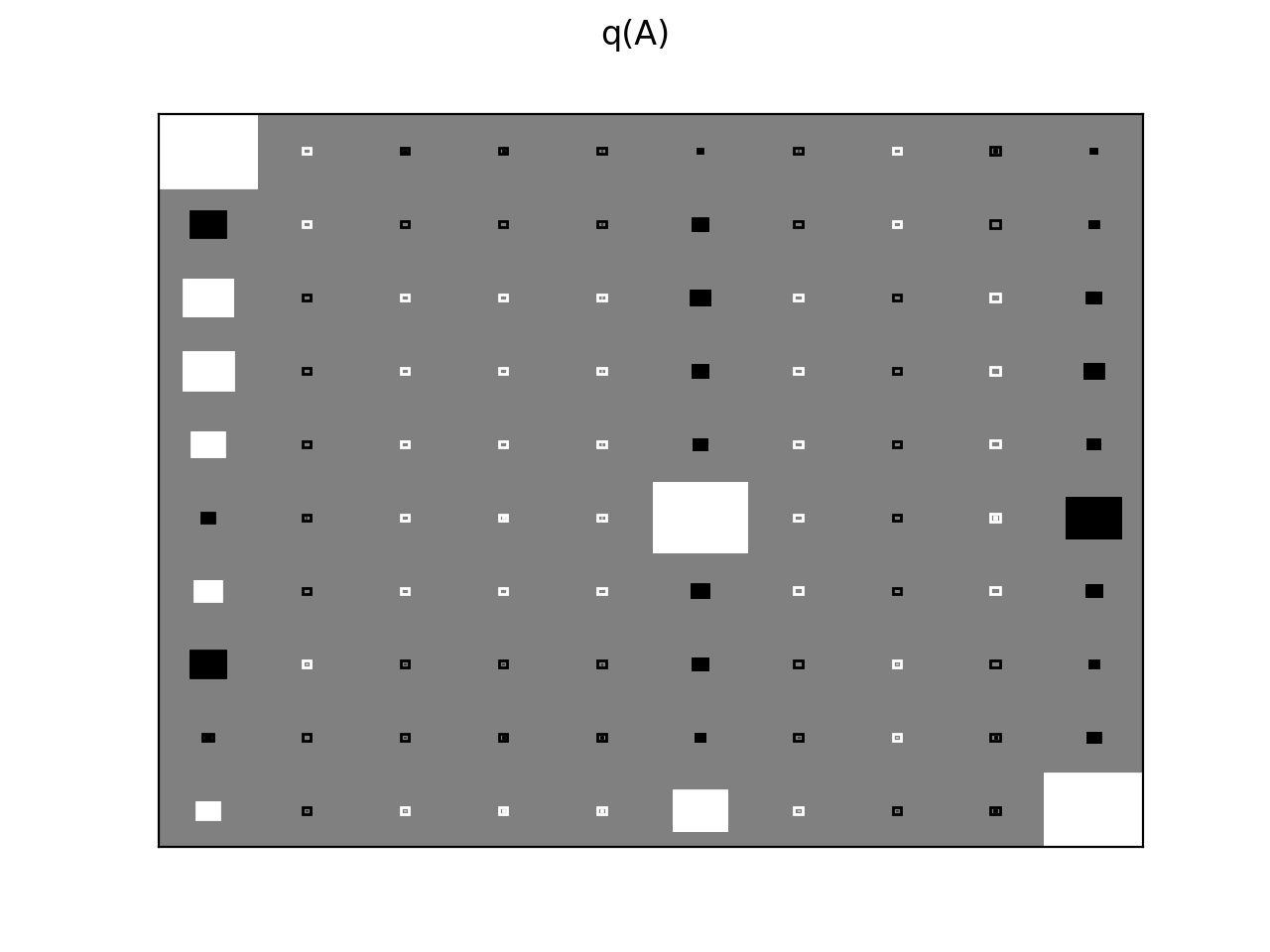
>>> A.set_plotter(bpplt.HintonPlotter())
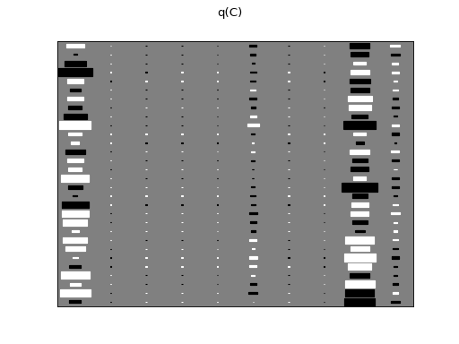
>>> C.set_plotter(bpplt.HintonPlotter())
>>> tau.set_plotter(bpplt.PDFPlotter(np.linspace(0.02, 0.5, num=1000)))

This enables plotting of the approximate posterior distributions during VB learning. The inference engine can be run using VB.update() method:

>>> Q.update(repeat=10)
Iteration 1: loglike=-1.439704e+05 (... seconds)
...
Iteration 10: loglike=-1.051441e+04 (... seconds)

The iteration progresses a bit slowly, thus we’ll consider parameter expansion to speed it up.

Parameter expansion¶

Section Parameter expansion discusses parameter expansion for state-space models to speed up inference. It is based on a rotating the latent space such that the posterior in the observation space is not affected:

$\mathbf{y}_n = \mathbf{C}\mathbf{x}_n = (\mathbf{C}\mathbf{R}^{-1}) (\mathbf{R}\mathbf{x}_n) \,.$

Thus, the transformation is $\mathbf{C}\rightarrow\mathbf{C}\mathbf{R}^{-1}$ and $\mathbf{X}\rightarrow\mathbf{R}\mathbf{X}$ . In order to keep the dynamics of the latent states unaffected by the transformation, the state dynamics matrix $\mathbf{A}$ must be transformed accordingly:

$\mathbf{R}\mathbf{x}_n = \mathbf{R}\mathbf{A}\mathbf{R}^{-1} \mathbf{R}\mathbf{x}_{n-1} \,,$

resulting in a transformation $\mathbf{A}\rightarrow\mathbf{R}\mathbf{A}\mathbf{R}^{-1}$ . For more details, refer to [6] and [7]. In BayesPy, the transformations are available in bayespy.inference.vmp.transformations:

>>> from bayespy.inference.vmp import transformations

The rotation of the loading matrix along with the ARD parameters is defined as:

>>> rotC = transformations.RotateGaussianARD(C, gamma)

For rotating X, we first need to define the rotation of the state dynamics matrix:

>>> rotA = transformations.RotateGaussianARD(A, alpha)

Now we can define the rotation of the latent states:

>>> rotX = transformations.RotateGaussianMarkovChain(X, rotA)

The optimal rotation for all these variables is found using rotation optimizer:

>>> R = transformations.RotationOptimizer(rotX, rotC, D)

Set the parameter expansion to be applied after each iteration:

>>> Q.callback = R.rotate

Now, run iterations until convergence:

>>> Q.update(repeat=1000)
Iteration 11: loglike=-1.010...e+04 (... seconds)
...
Iteration 58: loglike=-8.906...e+03 (... seconds)
Converged at iteration ...

Results¶

Because we have set the plotters, we can plot those nodes as:

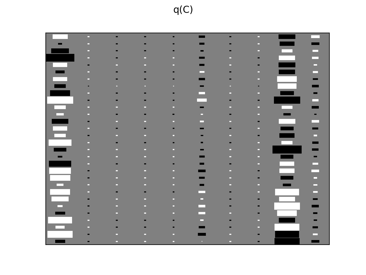
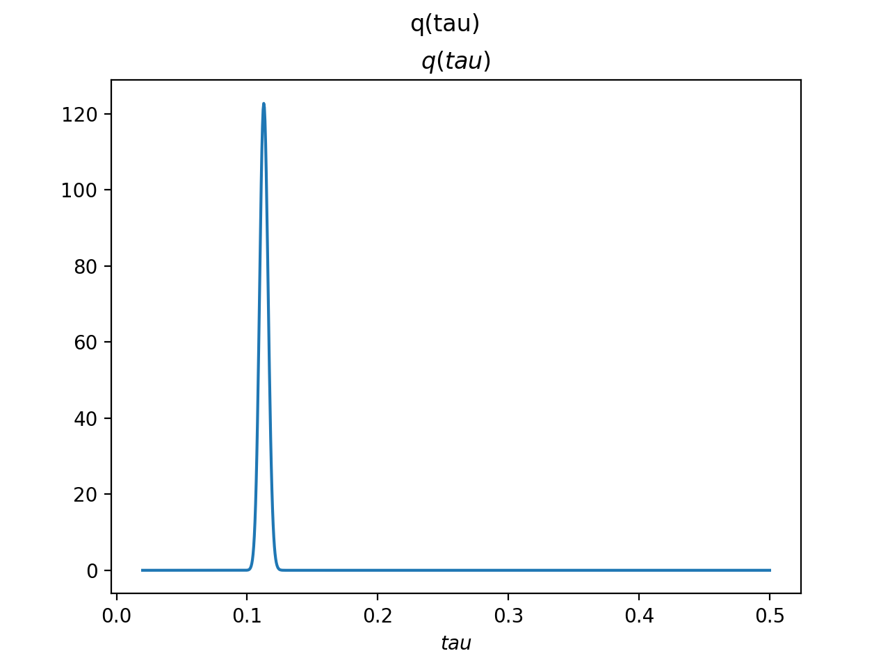
>>> Q.plot(X, A, C, tau)

(Source code)

../_images/lssm-1_00.png — (`png`, `hires.png`, `pdf`)¶

../_images/lssm-1_01.png — (`png`, `hires.png`, `pdf`)¶

../_images/lssm-1_02.png — (`png`, `hires.png`, `pdf`)¶

../_images/lssm-1_03.png — (`png`, `hires.png`, `pdf`)¶

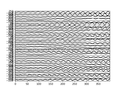
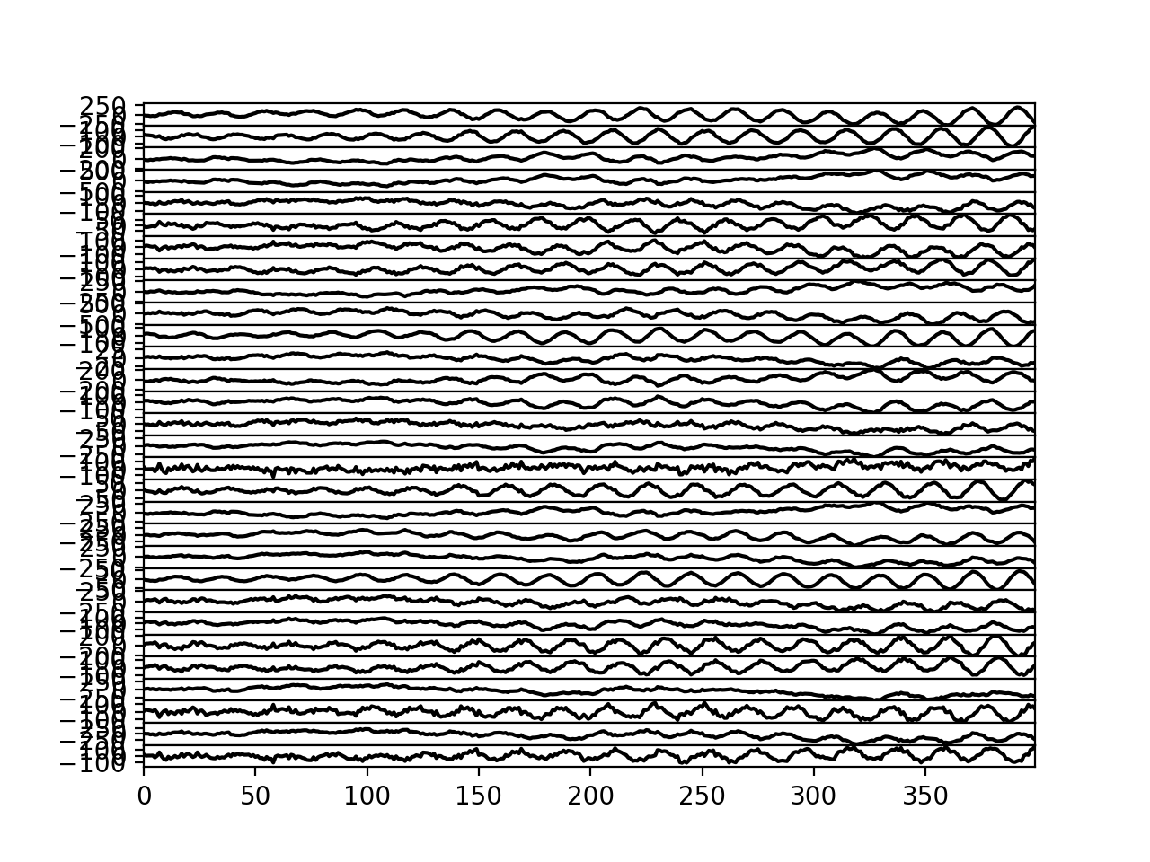
There are clearly four effective components in X: random walk (component number 1), random oscillation (7 and 10), and white noise (9). These dynamics are also visible in the state dynamics matrix Hinton diagram. Note that the white noise component does not have any dynamics. Also C shows only four effective components. The posterior of tau captures the true value $3^{-2}\approx0.111$ accurately. We can also plot predictions in the observation space:

>>> bpplt.plot(F, center=True)

(Source code, png, hires.png, pdf)

We can also measure the performance numerically by computing root-mean-square error (RMSE) of the missing values:

>>> from bayespy.utils import misc
>>> misc.rmse(y[~mask], F.get_moments()[0][~mask])
5.18...

This is relatively close to the standard deviation of the noise (3), so the predictions are quite good considering that only 20% of the data was used.

Linear state-space model¶

Model¶

Data¶

Inference¶

Parameter expansion¶

Results¶

BayesPy

Navigation

Related Topics