Principal component analysis

This example uses a simple principal component analysis to find a two-dimensional latent subspace in a higher dimensional dataset.

Data

Let us create a Gaussian dataset with latent space dimensionality two and some observation noise:

>>> M = 20
>>> N = 100

>>> import numpy as np
>>> x = np.random.randn(N, 2)
>>> w = np.random.randn(M, 2)
>>> f = np.einsum('ik,jk->ij', w, x)
>>> y = f + 0.1*np.random.randn(M, N)

Model

We will use 10-dimensional latent space in our model and let it learn the true dimensionality:

>>> D = 10

Import relevant nodes:

>>> from bayespy.nodes import GaussianARD, Gamma, SumMultiply

The latent states:

>>> X = GaussianARD(0, 1, plates=(1,N), shape=(D,))

The loading matrix with automatic relevance determination (ARD) prior:

>>> alpha = Gamma(1e-5, 1e-5, plates=(D,))
>>> C = GaussianARD(0, alpha, plates=(M,1), shape=(D,))

Compute the dot product of the latent states and the loading matrix:

>>> F = SumMultiply('d,d->', X, C)

The observation noise:

>>> tau = Gamma(1e-5, 1e-5)

The observed variable:

>>> Y = GaussianARD(F, tau)

Inference

Observe the data:

>>> Y.observe(y)

We do not have missing data now, but they could be easily handled with mask keyword argument. Construct variational Bayesian (VB) inference engine:

>>> from bayespy.inference import VB
>>> Q = VB(Y, X, C, alpha, tau)

Initialize the latent subspace randomly, otherwise both X and C would converge to zero:

>>> C.initialize_from_random()

Now we could use VB.update() to run the inference. However, let us first create a parameter expansion to speed up the inference. The expansion is based on rotating the latent subspace optimally. This is optional but will usually improve the speed of the inference significantly, especially in high-dimensional problems:

>>> from bayespy.inference.vmp.transformations import RotateGaussianARD
>>> rot_X = RotateGaussianARD(X)
>>> rot_C = RotateGaussianARD(C, alpha)

By giving alpha for rot_C, the rotation will also optimize alpha jointly with C. Now that we have defined the rotations for our variables, we need to construct an optimizer:

>>> from bayespy.inference.vmp.transformations import RotationOptimizer
>>> R = RotationOptimizer(rot_X, rot_C, D)

In order to use the rotations automatically, we need to set it as a callback function:

>>> Q.set_callback(R.rotate)

For more information about the rotation parameter expansion, see [7] and [6]. Now we can run the actual inference until convergence:

>>> Q.update(repeat=1000)
Iteration 1: loglike=-2.33...e+03 (... seconds)
...
Iteration ...: loglike=6.500...e+02 (... seconds)
Converged at iteration ...

Results

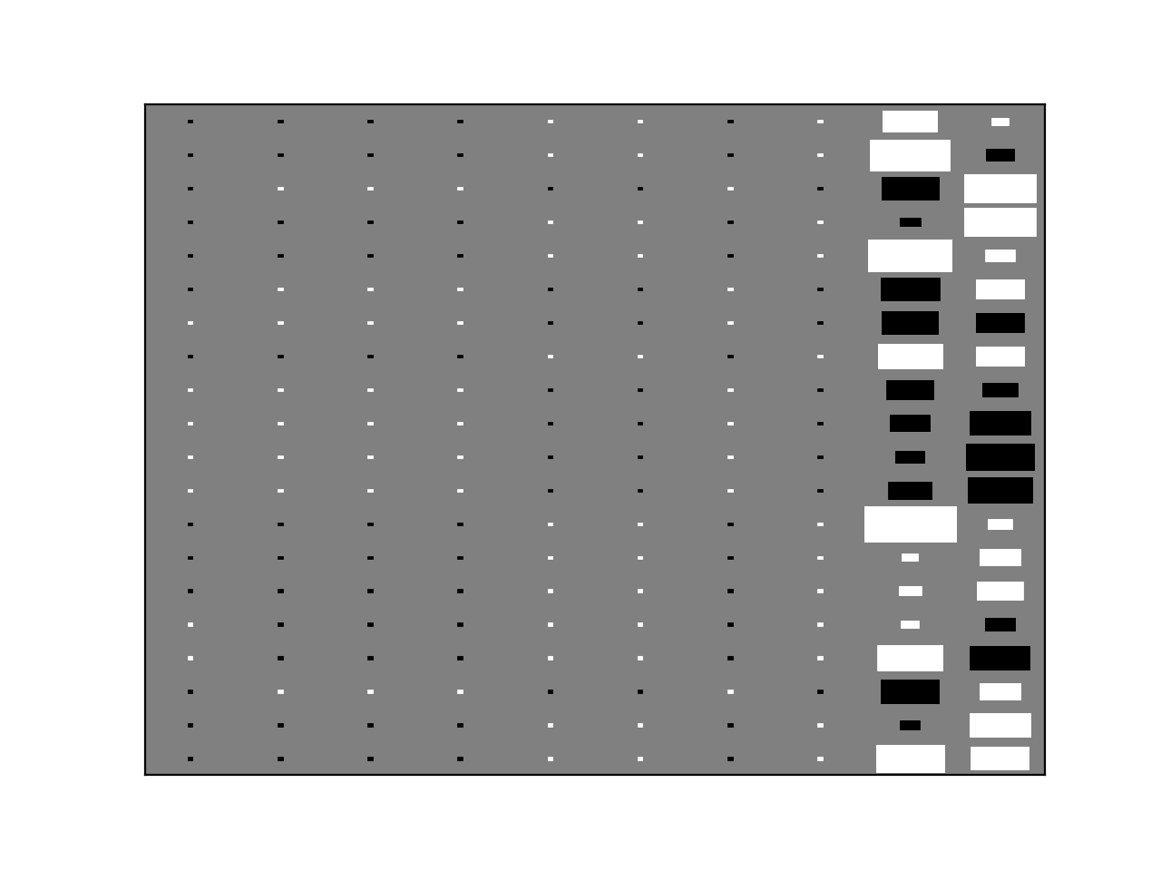
The results can be visualized, for instance, by plotting the Hinton diagram of the loading matrix:

>>> import bayespy.plot as bpplt
>>> bpplt.pyplot.figure()
<matplotlib.figure.Figure object at 0x...>
>>> bpplt.hinton(C)

(Source code, png, hires.png, pdf)

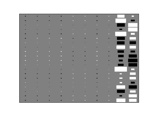
The method has been able to prune out unnecessary latent dimensions and keep two components, which is the true number of components.

>>> bpplt.pyplot.figure()
<matplotlib.figure.Figure object at 0x...>
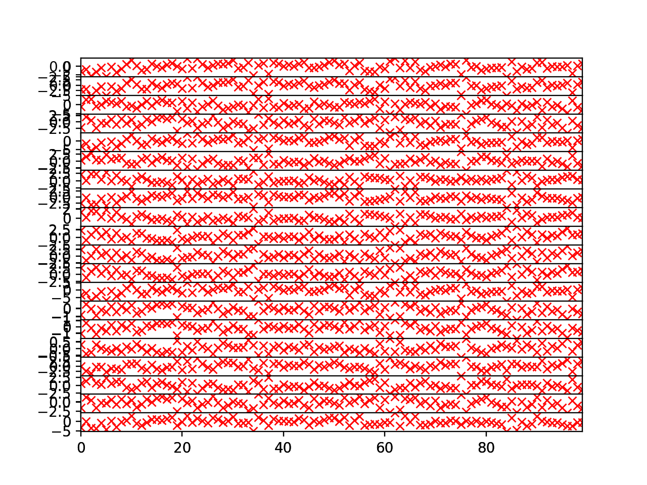
>>> bpplt.plot(F)
>>> bpplt.plot(f, color='r', marker='x', linestyle='None')

(Source code, png, hires.png, pdf)

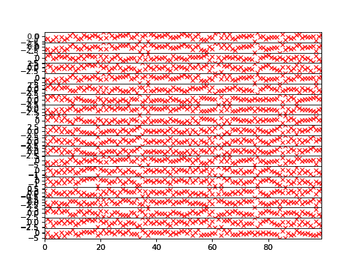
The reconstruction of the noiseless function values are practically perfect in this simple example. Larger noise variance, more latent space dimensions and missing values would make this problem more difficult. The model construction could also be improved by having, for instance, C and tau in the same node without factorizing between them in the posterior approximation. This can be achieved by using GaussianGammaISO node.